Ternary networks in SteadyCellPhenotype
Ternary models can represent biomolecular networks in a simple and intuitive manner by viewing the network in terms of a collection of logical rules. One can think of these models as an extension of Boolean models if simple logic is employed, but ternary models can also utilize more complicated rules and expressions. Each species in ternary network is represented by three states: 0, 1, and 2. Various assignments have been suggested for the states. For example, one possibility is to view 0 as false/inactive, 2 as true/active, and 1 as unknown, meaning that 1 can be either true/active or false/inactive. Another possibility is to think of these numbers as concentration levels of various proteins: low (0), normal (1) and high (2). Regardless of the labeling, the interactions in the network can be translated into functions over the finite field on three elements and then used to perform simulations, computations of the attractors, and visualizations of these attractors and trajectories.
An example of a biological network (or a graph) is depicted in Figure 1 below. This network is part of our previously published much larger network (see doi:10.1371/journal.pcbi.1005352 ). We have selected the iron homeostasis pathway to demonstrate the ideas and the terminology of this section. The underlying graph of this network is also a directed graph in the sense that each species is connected by an arc (edge) that has a direction, e.g., there is an arrow from TfR1 (transferrin receptor 1) to LIP (labile iron pool). In addition, in this network the graph is a signed graph, that is, each connection from one species to the next is either positive (activation - a blue arc with an arrow head) or negative (inhibition - an orange arc with a hammer head). We would like to note, that edges joining species do not have to be signed, but in most applications, majority of connections will be positive or negative.

Local activation functions
The next step in model building is to define a local activation function for each node in the network. The value of each local activation function depends on its input nodes (species) and their current state. This can be accomplished in multiple ways (i) using an analog to the Boolean formalism, (ii) tables and (iii) functions over finite field on three elements. These are not the only possibilities. Here we describe the first possibility and just mention the second (our future editions will include generation of functions from tables directly). As for the third option and others, our browser based interface SteadyCellPhenotype is capable of reading any input function over a finite field on three elements, thus allowing the user to explore any type of ternary network.
A local activation function for a node \(v\) is often denoted in literature by \(f_v\). If the node \(v\) has multiple input nodes \( w_1, w_2, \dots, w_k \), then this function is written as \( f_v(w_1, w_2, \dots, w_k)\). Using this notation and Figure 1 activation function, for example, for LIP is then \(f_{LIP}(TfR1, Fpn, Ft)\). To make notations simpler, SteadyCellPhenotype allows the user to replace the bulky notation \(f_{LIP}(TfR1, Fpn, Ft)\) by simply typing \(LIP.\)
Now suppose, that a node in the network only has one input (e.g., IRP1 and IRP2 in Figure 1) and it is clear from the biological evidence if the regulation is positive or negative. In this case, one can use simple relations as depicted by the tables below.
| \(X\) | \(f_Y(X)\) |
|---|---|
| 0 | 0 |
| 1 | 1 |
| 2 | 2 |
| \(X\) | \(f_Y(X)\) |
|---|---|
| 0 | 2 |
| 1 | 1 |
| 2 | 0 |
Local activation functions depicting these tables are then:
Since \(-1 \bmod 3 = 2\), then the equation for inhibition can also be written as \(f_Y(X) = 2+2X\). Note that the table for inhibition just reverses the values and so can be considered as an analog of the Boolean NOT gate. The user may then write the local activation function for inhibition in several ways, including algebraic forms as well as using the included not function.
When a node has two inputs (e.g., TfR1, Fpn and Ft in Figure 1) then the local activation functions may also be defined using the max or min operators (see Tables below).
| \(X\) | \(Y\) | \(f_Z(X,Y)\) |
|---|---|---|
| 0 | 0 | 0 |
| 0 | 1 | 1 |
| 0 | 2 | 2 |
| 1 | 0 | 1 |
| 1 | 1 | 1 |
| 1 | 2 | 2 |
| 2 | 0 | 2 |
| 2 | 1 | 2 |
| 2 | 2 | 2 |
| \(X\) | \(Y\) | \(f_Z(X,Y)\) |
|---|---|---|
| 0 | 0 | 0 |
| 0 | 1 | 0 |
| 0 | 2 | 0 |
| 1 | 0 | 0 |
| 1 | 1 | 1 |
| 1 | 2 | 1 |
| 2 | 0 | 0 |
| 2 | 1 | 1 |
| 2 | 2 | 2 |
Note that SteadyCellPhenotype's max and min operators support exactly two arguments. One can also combine operators, using the not operator inside the max and min. For example, if X activates node Z but Y inhibits node Z then a possible update rule could be \(f_Z(X,Y)=\min(X,\mathrm{not}(Y)))\).
If nontraditional activation, inhibition, or any other modulations are required, then the user may enter any combination of algebraic or max/min/not expressions and SteadyCellPhenotype will evaluate the corresponding function modulo 3.
For nodes with more than two inputs, any composition of the max, min, and not operators are possible. The not operator will always take a single expression as input and the max and min operators take two comma delimited arguments. Similar to the cases above, other expressions can be used as well among input nodes. Internally, max and min operators are recoded as polynomials of degree four when necessary for algebraic computations:
Note: Unlike variable names, the names of the max, min and not operators are case insensitive and either lower case, all caps, or a combination of cases can be used to enter these functions.
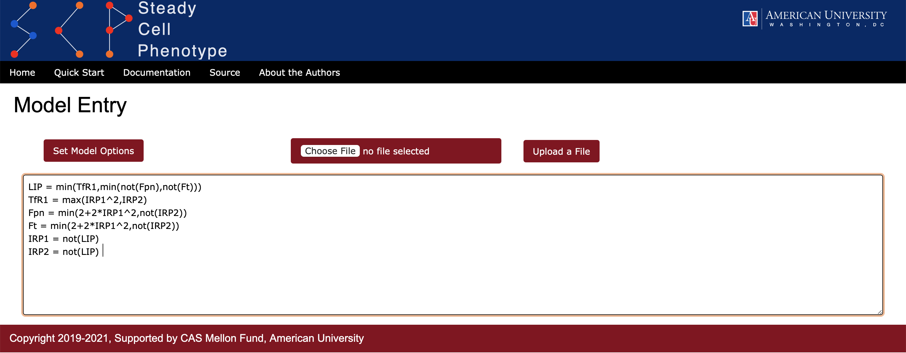
Example: iron homeostasis pathway
Using the graph in Figure 1 and rules as described in doi:10.1371/journal.pcbi.1005352 we can write local activation functions for this portion of the network. Note that IRP1 has an adjusted rule (see discussion on pages 16-17 of the article mentioned above). Syntax and the actual entry within an application (Figure 2) are shown below. Note, the user also has an option to upload the file in text (.txt) format.
Continuity
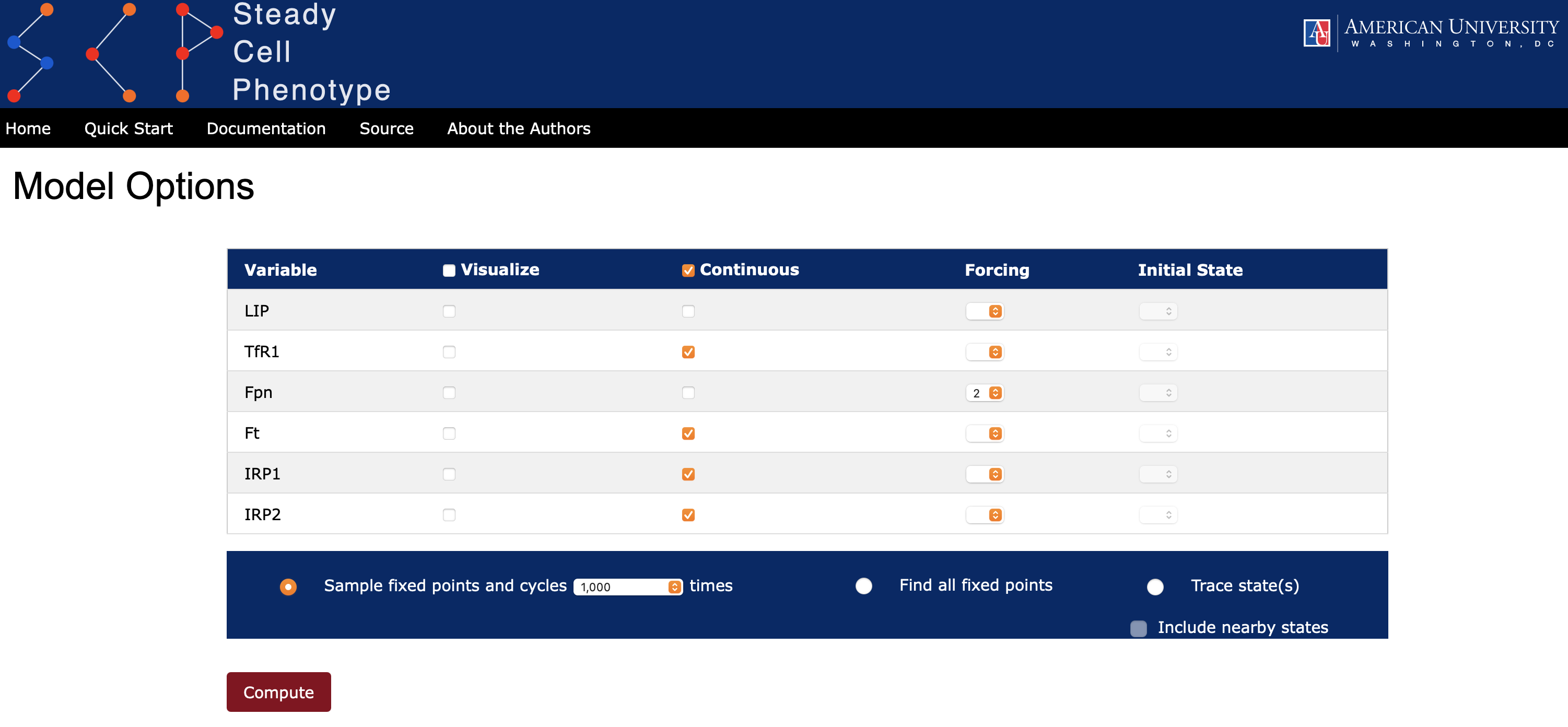
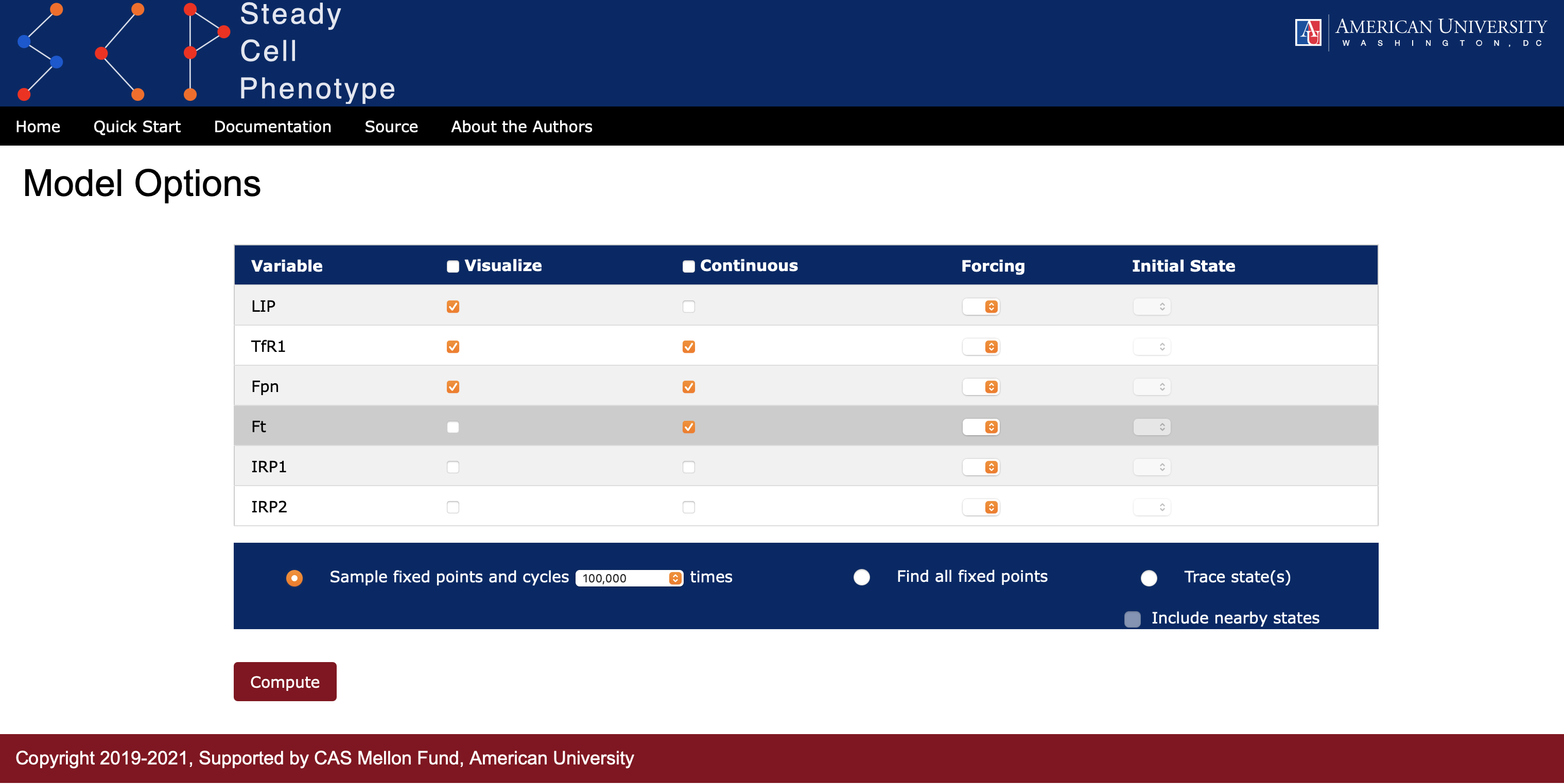
In Boolean networks there is a single scale of change for each node. However, in ternary networks there are two possible scales: a jump \(\pm1\) or \(\pm 2\). This means that a node can have a "discontinuous" change, for example from low (0) to high (2), in a single time step. If the user wishes to ensure that all or some nodes change by at most one unit then one can select an option Continuous for the variables (see Figure 3). Internally, continuity is applied to each update rule as follows:
- the local activation function \(f_X\) is computed for the variable \(X\) and compared to the current state of the variable,
- if the current state of \(X\) is the same as \(f_X\) or differs from \(f_X\) by one unit only, then the value assigned to the variable is \(f_X\), and
- if the current state of \(X\) and \(f_X\) differs by \(\pm2\), then the value of \(X\) at the next time step moves by 1 in the direction of \(f_X\).
State Space: attractors
In the current version of SteadyCellPhenotype, all nodes in the network are on a synchronous update schedule, where all values are updated simultaneously. This implies that trajectories are deterministic and each state of the network will belong to the basin of attraction of only one attractor: a fixed point or cyclic attractor.
Fixed Points can be computed using two different options.
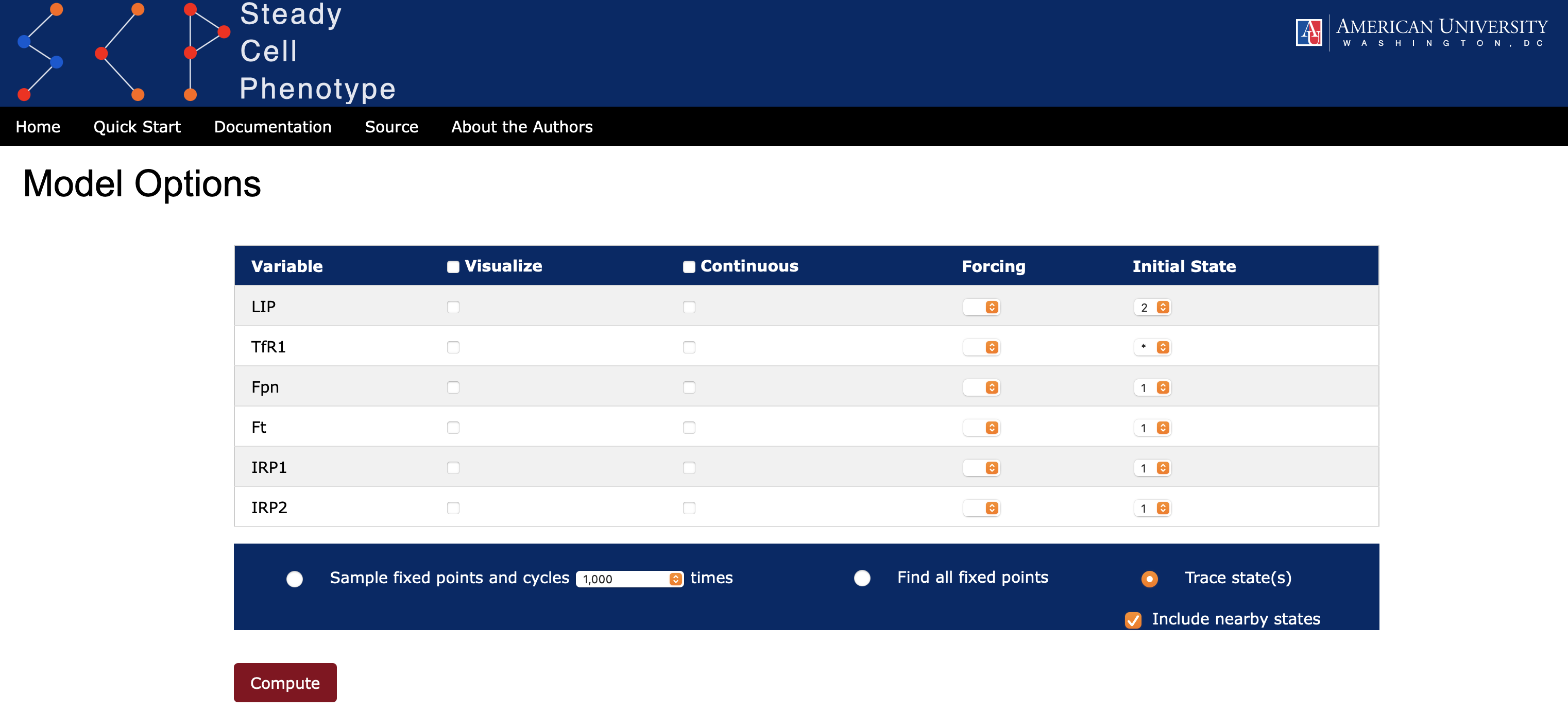
- Selecting the radio-button Find all fixed points (see Figure 3). In this case SteadyCellPhenotype will compute all fixed points analytically. If the model has no fixed points then a Message with the text indicating that there are no fixed points will be displayed.
- Another option to find some of the fixed points is by selecting the radio-button Sample fixed points and cycles. Here the user can select from the dropdown list the number of random initial states from which the trajectory will be computed.
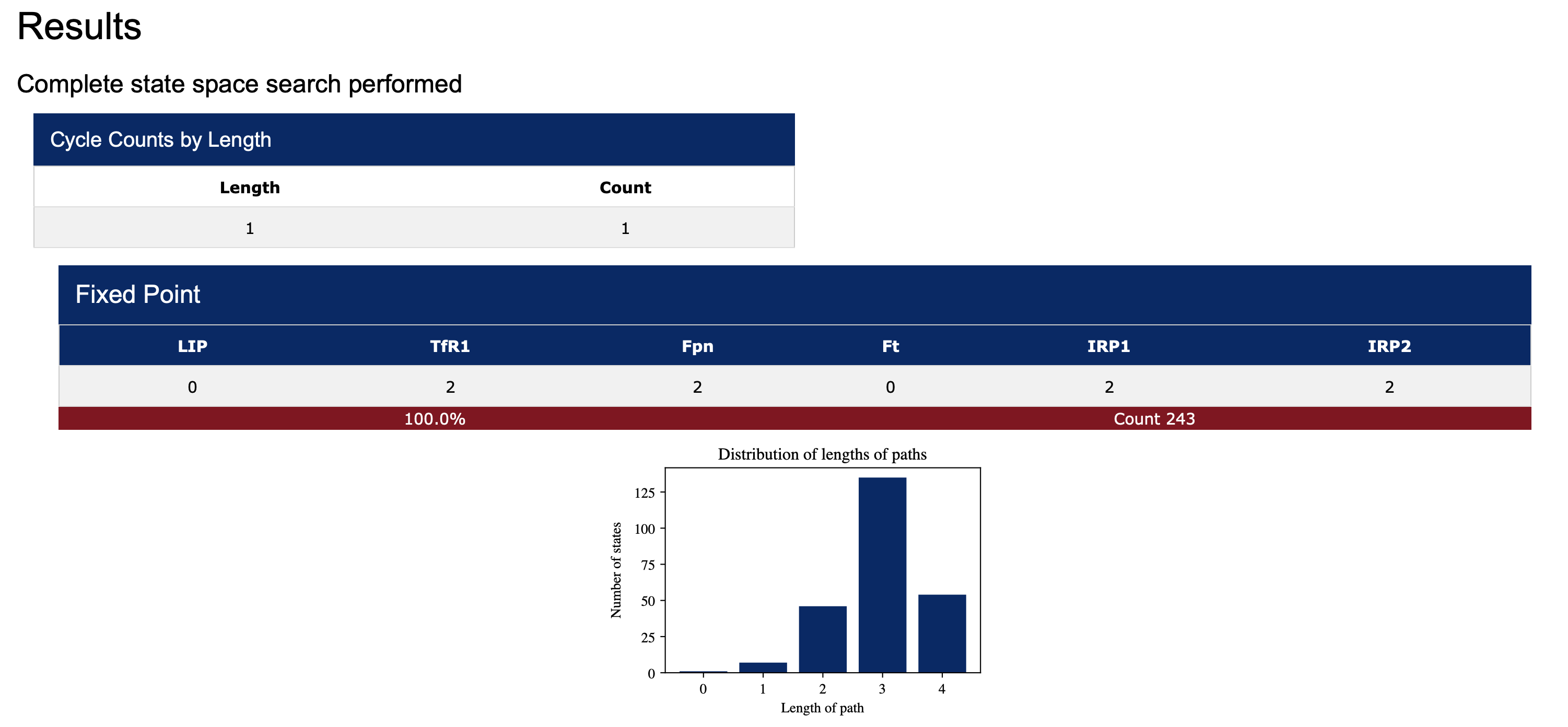
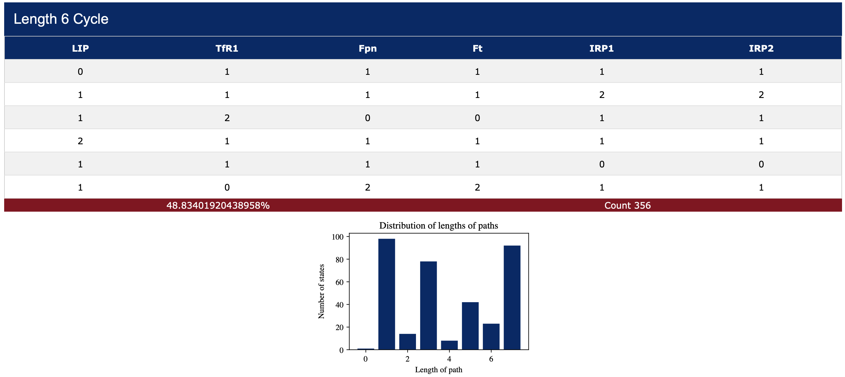
When the radio-button Sample fixed points and cycles is selected, the length of each trajectory leading to an attractor for each random start is recorded. A histogram, summarizing a distribution of the path lengths, is displayed below each attractor (see Figure 4). Attractors can be saved in a comma-separated values (csv) format. All images also have a save button.
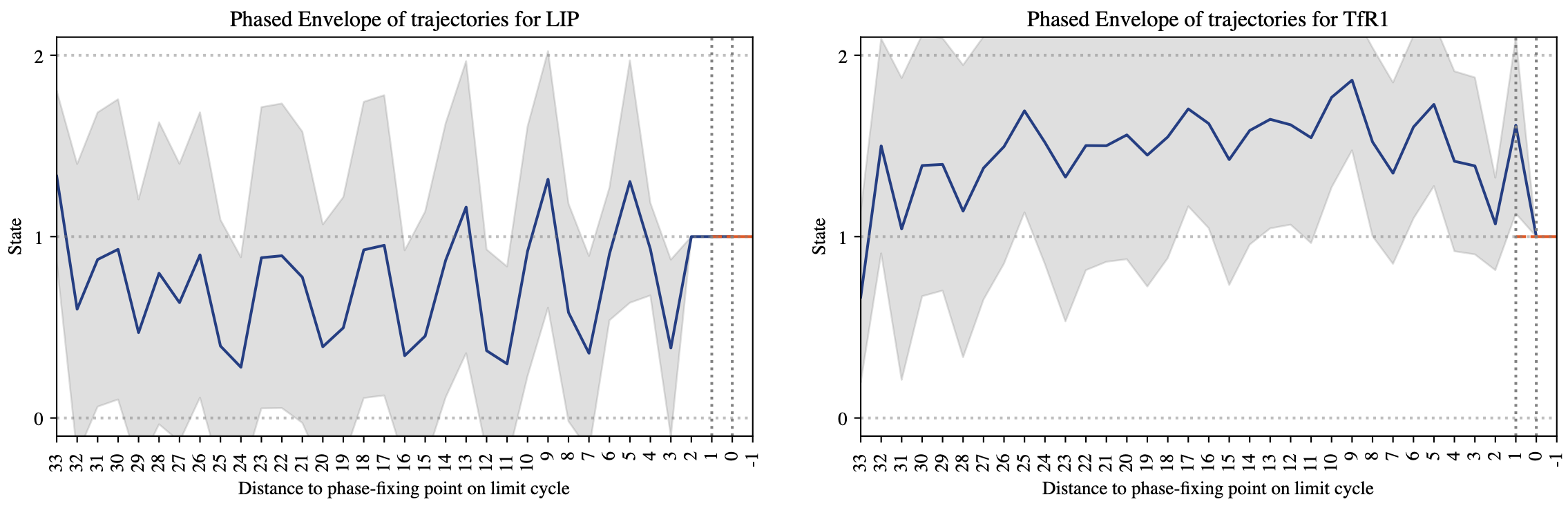
Additionally, the user can select the Visualize option for all or some of the variables (one can see this option in Figure 3). When this option is selected then SteadyCellPhenotype will collect additional statistics. In particular, for each random starting state a trajectory (path) is recorded. The collection of all these trajectories are then aligned on the right to ensure that they all arrive at the same time at the fixed point or at a specified point on their cyclic attractor. The image in Figure 5 displays the mean value and standard deviation of the variable states along these trajectories. This feature is useful in demonstrating, for example, if a biological species of interest (LIP) had a cyclic behavior before entering a fixed point.
Tracing a Specific State
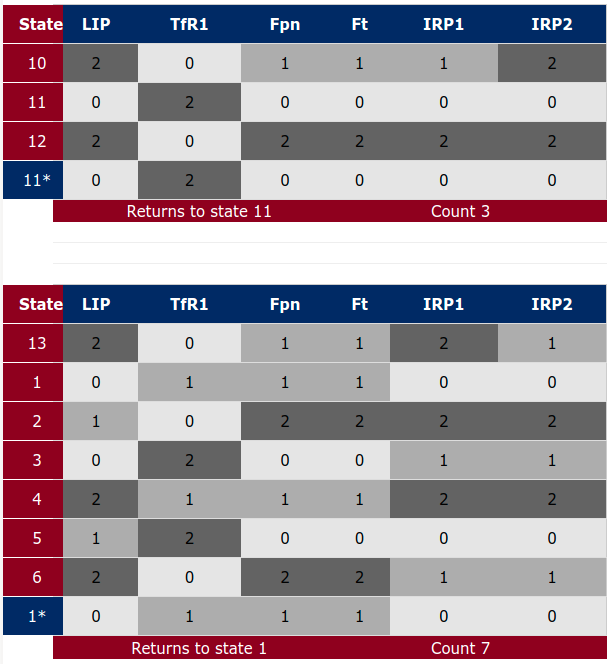
SteadyCellPhenotype offers an option to trace a specific state by selecting the Trace state(s) radio button. This allows the user to investigate the evolution of interesting states and visualize trajectories via a graph. Under the Initial State option the user can choose from a dropdown list the values 0, 1, 2, or * (see Figure 6). The symbol asterisk (*) means that all states for this particular species will be considered. If the user would like to investigate nearby states around a specific point of interest, then checking the box Include nearby states will include the evolution of trajectories from states that are Hamming distance one from the specified point, i.e., all states that differ from the specified state by one unit for exactly one species. SteadyCellPhenotype will display a heatmap that records the evolution of trajectories and a directed graph summarizing these paths (see Figure 7). The option to save the graph and heatmap are available. The values in the heatmap will be saved in a comma-separated values (cvs) format.

Note: for small models selecting asterisk (*) for all species will result in the computation of the entire state space. Using this option for large models is not advisable. The complete state space for our running example is displayed in Figure 8, below.

Knockout and Overexpression Experiments
SteadyCellPhenotype has an option to simulate the effects of knockout (k/o) or overexpression (o/e) by using an option Forcing and selecting a value from the dropdown list 0, 1, or 2 (Figure 9). This will set the update rule to a constant value of the selected species. Attractors then can be computed as described in State Space section.